Searle’s Chinese Room, Reductionism, and Gaussian Mixture Models

Recently, I delved into John Searle’s Chinese Room argument, a thought experiment that challenges the notion that a computer running a program can possess a mind, consciousness, or genuine understanding. Searle presented this argument in his 1980 paper “Minds, Brains, and Programs” to counter the claims of strong artificial intelligence, which posits that appropriately programmed computers can have genuine mental states.
Searle’s Chinese Room Thought Experiment
-
The Room: A person (Searle) is inside a room, isolated from the outside world except for a slot through which symbols can be passed in and out.
-
Chinese Characters: People outside the room, who understand Chinese, pass slips of paper with Chinese characters into the room.
-
The Rulebook: Inside the room, Searle has a rulebook written in English that contains instructions for manipulating the Chinese characters purely syntactically (i.e., based on their shapes, not their meanings). By following these instructions, he can produce appropriate Chinese characters in response, which he then passes back out of the room.
-
Simulation of Understanding: To the people outside, it appears as though there is someone inside the room who understands Chinese because the responses are appropriate and contextually correct.
Searle argues that despite his ability to manipulate Chinese symbols to produce correct responses, he does not understand Chinese. He is merely following syntactical rules without comprehending the meaning (semantics) of the symbols. Therefore, even though the system (Searle + rulebook) can produce intelligent behaviour that simulates understanding, there is no genuine understanding or consciousness involved.
For those interested in exploring this thought experiment further, an excellent resource can be found at the Stanford Encyclopedia of Philosophy. This thought experiment naturally leads to broader questions about complexity of systems:
-
Are complex systems merely the sum of their parts?
-
Do emergent properties arise, and if so, what are the causal relationships within the hierarchy of complex systems?
-
What methods can we use to study these relationships?
As discerning readers may have observed, these inquiries delve into the philosophical domains of reductionism and emergentism.
Reductionism : Reductionism is the idea that complex systems can be understood by breaking them down into their simpler, fundamental parts. It interprets a complex system as the sum of its parts.
Emergentism : Emergentism posits that a system exhibits properties that arise from the interactions of its parts but are not reducible to those parts. These properties are considered emergent because they are new outcomes from the system’s interactions.
In seeking real-world applications, I couldn’t resist examining how these concepts apply to financial markets. Financial markets can be seen through the lens of both schools of thought: as emergent phenomena resulting from a complex network of agents influenced by cognitive biases and social dynamics, and from a reductionist perspective, where quantitative methods such as factor models and time series analysis are used to investigate relationships between market factors and returns.
To navigate this dichotomy, this articles explores an approach that, I think, lies somewhere in the middle: Gaussian Mixture Models (GMMs).
A GMM is a probabilistic framework that represents a distribution of data points as a mixture of multiple Gaussian (normal) distributions. Each Gaussian distribution in the mixture signifies a cluster or component of the data, and the overall model combines these distributions to capture the complex, multimodal nature of the data. GMMs are extensively used in statistics, machine learning, and data analysis for tasks like clustering, density estimation, and pattern recognition.
Why GMMs
Before delving deeper into GMMs, here are a few reasons why I think that these models are intriguing in the context of our discussion so far:
-
Simplification of Complex Data: Starting with complex data, such as daily financial index returns, GMMs reduce complexity by assuming the returns are a weighted average of different Gaussian distributions, helping account to fat tails and/or regime changes that are frequently observed in such data.
-
Weak Emergence: After fitting our training data to estimate the model parameters, the actual returns can be considered weakly emergent. This means that while we posit that final returns stem from lower-level interactions, we acknowledge this to be only probabilistically true and the actual returns might be a weighted average function of some other specification. In other words, we can only probabilistically estimate the actual returns belonging to one regime (Gaussian distribution) or another.
Illustrative Scenarios for GMM Application
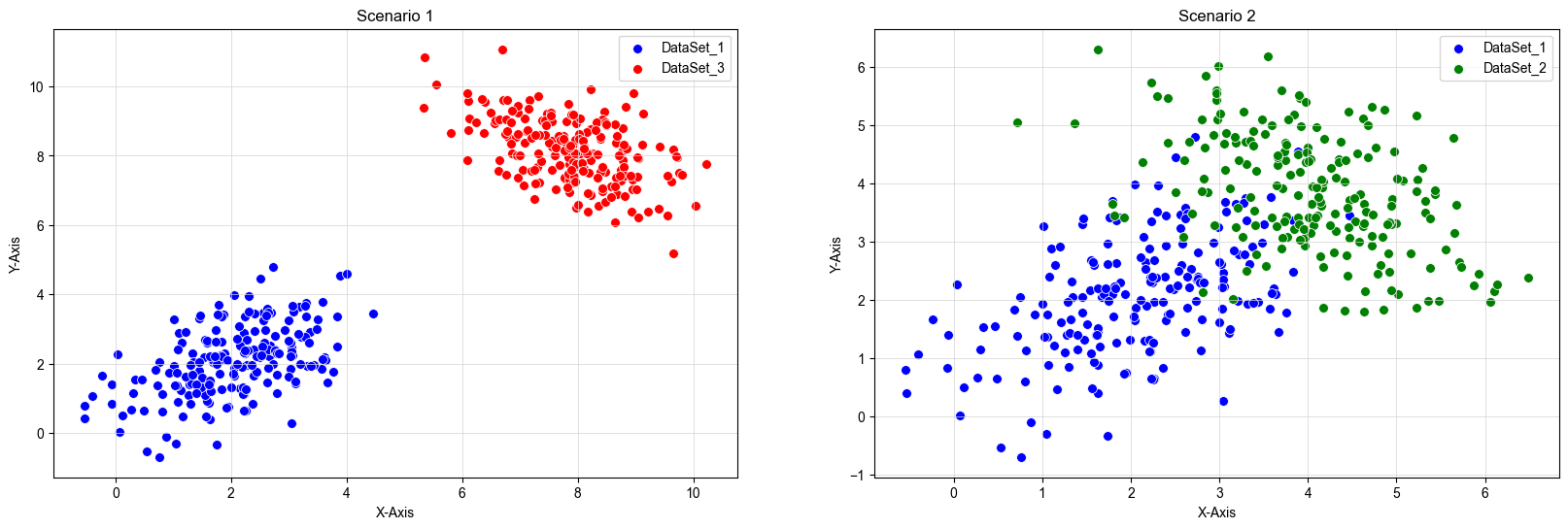
To provide a more intuitive understanding of where GMMs excel, consider the following scenarios in Image 1:
-
Scenario 1: The data clearly appears in two distinct clusters. In such cases, given the clear distinction, a different algorithm might be preferable due to the obvious separation of the two datasets.
-
Scenario 2: The data points are in close proximity. As such, making binary cluster classifications is neither straightforward nor appropriate. This is where GMMs shine, allowing us to capture the nuances in the data distribution.

DataSet_1: mean: [2 , 2] ; covariance matrix: [[1.0 , 0.5] , [0.5 , 1.0]]
DataSet_2: mean: [4 , 4] ; covariance matrix: [[1.0 , -0.5] , [-0.5 , 1.0]]
DataSet_3: mean: [8 , 8] ; covariance matrix: [[1.0 , -0.5] , [-0.5 , 1.0]]
With these initial conditions in mind, let’s outline the step-by-step approach of the GMM algorithm:
For our initial test, let’s create some synthetic data. We will draw from two bivariate normal distributions to create our data. For the purpose of this exercise, this is the same dataset that you see in Image 1, Scenario 2 above.
# Parameters for the synthetic data
np.random.seed(0)
mean1 = np.array([2, 2])
cov1 = np.array([[1, 0.5], [0.5, 1]])

mean2 = np.array([4, 4])
cov2 = np.array([[1, -0.5], [-0.5, 1]])

# Generate data
data1 = np.random.multivariate_normal(mean1, cov1, 200)
data2 = np.random.multivariate_normal(mean2, cov2, 200)
data = np.vstack((data1, data2))
Initialization involves setting initial values for the parameters of the Gaussian components. These parameters include the means, covariances, and mixing coefficients.
-
Means: Randomly select initial mean values for each Gaussian component. One common approach is to choose k data points randomly as initial means.
-
Covariances: Initialize the covariance matrices for each component. A simple approach is to use the overall covariance of the data for each component.
-
Mixing Coefficients: Set the initial mixing coefficients, which are typically initialized equally, summing to 1.
def initialize_parameters(data, k):
    n, d = data.shape
    means = data[np.random.choice(n, k, False)]
    covariances = np.array([np.cov(data, rowvar=False)] * k)
    mixing_coefficients = np.ones(k) / k
    return means, covariances, mixing_coefficients

# Number of components (regimes)
k = 2

# Initialize parameters
means, covariances, mixing_coefficients = initialize_parameters(data, k)
The EM algorithm iteratively refines the parameters of the GMM to maximize the likelihood of the data. It alternates between two main steps: Expectation (E-step) and Maximization (M-step).
E-Step: Expectation Step
In the E-step, calculate the responsibilities, which represent the probability that each data point belongs to each Gaussian component.
Calculate Responsibilities: For each data point and each Gaussian component, compute the probability of the data point given the component’s parameters (mean and covariance). Then, weight this probability by the component’s mixing coefficient.
Normalize Responsibilities: Ensure the responsibilities for each data point sum to 1 across all components. This normalization gives the posterior probabilities that each data point was generated by each component.
#E-Step: Expectation Step
def e_step(data, means, covariances, mixing_coefficients):
    n, d = data.shape
    k = means.shape[0]

    responsibilities = np.zeros((n, k))

    for i in range(k):
        responsibilities[:, i] = mixing_coefficients[i] * multivariate_normal.pdf(data, mean=means[i], cov=covariances[i])

    responsibilities = responsibilities / responsibilities.sum(axis=1, keepdims=True)

    return responsibilities
M-Step: Maximization Step
In the M-step, update the parameters of the Gaussian components using the responsibilities computed in the E-step.
Update Means: Compute the new mean of each Gaussian component as the weighted average of the data points, where the weights are the responsibilities.
Update Covariances: Update the covariance matrix for each component based on the weighted sum of the outer products of the deviations of the data points from the new means.
Update Mixing Coefficients: Compute the new mixing coefficients as the average responsibility of each component.
#M-Step: Maximization Step
def m_step(data, responsibilities):
    n, d = data.shape
    k = responsibilities.shape[1]

    nk = responsibilities.sum(axis=0)
    means = np.dot(responsibilities.T, data) / nk[:, np.newaxis]
    covariances = np.zeros((k, d, d))

    for i in range(k):
        diff = data - means[i]
        covariances[i] = np.dot(responsibilities[:, i] * diff.T, diff) / nk[i]

    mixing_coefficients = nk / n

    return means, covariances, mixing_coefficients
Repeat the E-step and M-step until the parameters converge. Convergence is typically defined as the point where changes in the parameter values fall below a predetermined threshold, or the improvement in the likelihood of the data given the model becomes negligible.
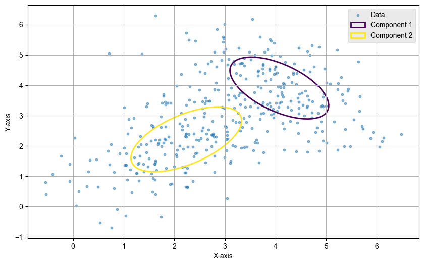
Image 2 effectively illustrates how the Gaussian Mixture Model has decomposed the initial (complex) data into simpler Gaussian components, each characterised by its mean, covariance, and orientation, providing insights into the underlying structure of the dataset.

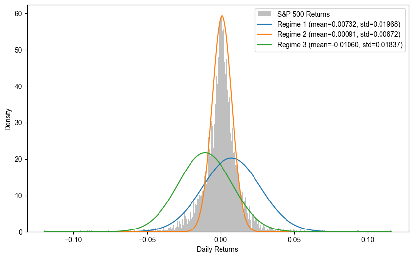
As an extension of this exploration, I also proceeded to analyze daily data from the S&P 500 index, applying the Gaussian Mixture Model to identify potential market regimes based on daily return data. The model successfully segmented the returns into three distinct regimes. Image 3 compares the empirical distribution of daily S&P 500 returns with the pdfs of the identified regimes by the GMM.

Conclusion
What began with a casual encounter with John Searle’s Chinese Room argument evolved into a philosophical exploration of the inherent tension between reductionism and emergence. While reductionism seeks to explain complex systems through their constituent parts, offering clear, definable relationships, emergentism, posits that new properties arise from the interactions within a system, properties not evident from the parts alone. Financial markets exemplify this philosophical tension. They are shaped by individual actions and interactions (reductionist view) but also display patterns and behaviors that emerge from the collective (emergent view).
For this article, I thought that GMMs were a neat way to explore the interplay between these schools of thought, decomposing complex data distributions into simpler Gaussian components and capturing the multifaceted nature of financial returns. By assuming returns result from a mixture of different regimes, GMMs enable a probabilistic approach to understanding market behaviour.
Code on GitHub.
Notes and References:
Minds, brains, and programs. John Searle - 1980 - Behavioral and Brain Sciences 3 (3):417-57.
- https://en.wikipedia.org/wiki/Reductionism
- https://en.wikipedia.org/wiki/Emergentism
- https://plato.stanford.edu/archIves/spr2010/entries/chinese-room/
- https://scikit-learn.org/stable/modules/generated/sklearn.mixture.GaussianMixture.html
- https://medium.com/@juanc.olamendy/understanding-gaussian-mixture-models-a-comprehensive-guide-df30af59ced7